Container Forming Simulation: The world is 3D
The real world is 3-D and nearly all containers produced have an unsymmetrical thickness distribution, even though the mold shape is axis-symmetric. In order to reduce the container weight or to achieve the increasing product quality by simultaneously reducing the costs it is fundamental to understand all mechanisms in glass forming processes.
Nogrid provides CFD (Computational Fluid Dynamics) simulation software developed especially for the container glass industry. Nogrid software can compute glass forming processes in full 3D and allows simulating all kinds of glass forming processes, amongst others for container glass:
- BB (Blow and Blow)
- PB (Press and Blow or Wide Mouth PB)
- NNPB (Narrow Neck Press and Blow)
In this paper the focus of attention lay on the glass forming, that means on the flow of the glass and for that reason the blank mold and the blow mold are replaced by approximate models.
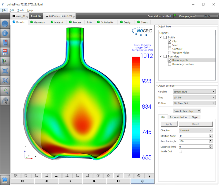
Figure 1: Result view of non axis-symmetric container
Figure 2 shows schematically the process steps that occur during the BB process, which was used in this investigation.
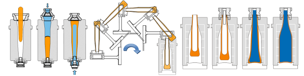
Figure 2: Schematic steps during BB process
The real world is 3-D and nearly all containers produced do have unsymmetrical thickness distribution, even though the mold shape is axis-symmetric. Simulation helps to understand and classify all mechanisms or effects which are responsible for unsymmetrical thickness distribution. Some mechanisms are hidden and coupled with each other and therefore it is very difficult to distinguish between them by experiments.
For instance, when one experiences a certain unexpected container wall thickness distribution (e.g. too much glass in the neck area), it is sometimes not clear, what the reasons are:
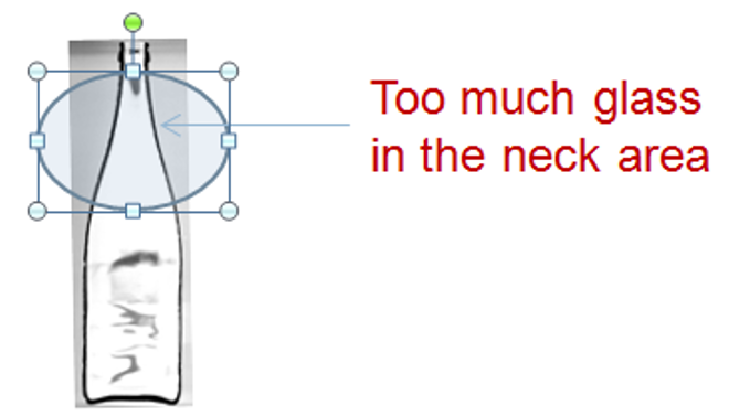
Cross section of container produced
- neck mold area too cold
- glass contact time too long
- gob temperature too low
- gob shape not correct
- or other causes.
In production one cannot simply increase the gob temperature, because also the gob shape will change in that case. That means one cannot distinguish what is the effect of temperature and what is the effect of gob shape. In simulation we can change the gob temperature and the gob shape remains the same. Thus, with computer simulation one can investigate each cause of defect independently from others and as a result one is able to investigate the dependencies step by step.
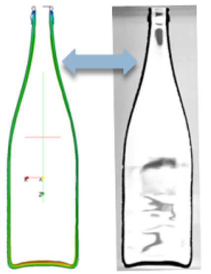
Comparison simulation - real
The most sensible material property for the glass forming process is the viscosity, which depends on temperature. Unfortunately glass temperatures are often entirely unknown and can be measured only with considerable effort. For that reason one important question very often is: What is the influence of the gob temperature on the container wall thickness distribution and what happens if the temperature distribution within the gob is not homogeneous? Beside inhomogeneous temperatures a non-symmetric gob load is also a major reason for an irregular wall thickness distribution. In this paper we will give some answers to these questions. As in reality, the simulation starts with gob loading and ends at take out. All process steps are integrated into one computer model and all walls are switched on and off at the corresponding time step given by the IS machine time data: The walls for the plunger, blank mold, blank mold bottom and final mold are combined to one single geometrical model. The software switches the corresponding faces on and off according to the IS time data.
Theory and Data
We solve the complete Navier-Stokes equations (continuity equation, velocity equations and energy equation) within the fluid. The glass viscosity depends on temperature as shown in Figure 3.
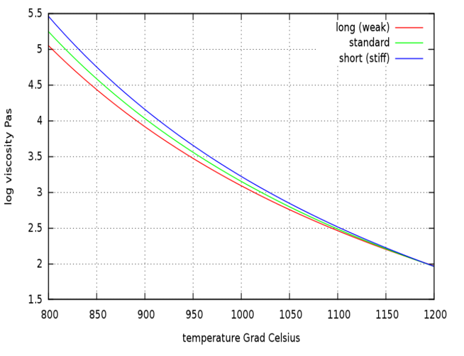
Figure 3: Viscosity depends on temperature
In the container glass industry the glass composition and therefore the glass properties can vary, but usually soda lime silica glass is used. We used the standard container glass for the computations in this paper. The blank mold, the blow mold and the plug are replaced by an approximate heat flux boundary condition
Q = h A ( Tglass-Tmold )
h is the heat transfer coefficient, T is the glass temperature at the interface glass-mold and Tmold is the temperature of the mold. The heat transfer coefficient h used is constant over time, but if better experimental data is available this can be modified easily. Two containers are considered for this investigation (see Figure 4 ); one has an axis-symmetric shape (C1) and the other not (C2).

Figure 4: Shape of containers used for investigation
We investigated the following conditions for both containers and all simulations are obtained by full 3-D computations:
- Symmetrical loading with homogeneous gob temperature
- Loading with homogeneous gob temperature, but the initial gob position is displaced from the center axis
- Gob loading position is centered, but the initial gob temperature is non-homogeneous.
Results
The conditions for the container C1 are:
Case C1-0
Symmetrical loading with homogeneous gob temperature
Case C1-1
Loading with homogeneous gob temperature, but the initial gob position is 2 mm displaced from the center axis.
Case C1-2
Gob loading position is centered, but the initial gob temperature is non-homogeneous. The gob temperature is 1163 °C in the center and decreases to 1126 °C on left side and increases to 1199 °C on the right side (see Figure 9). Thus, the maximum temperature difference in the gob is ∆T= 72 °C.
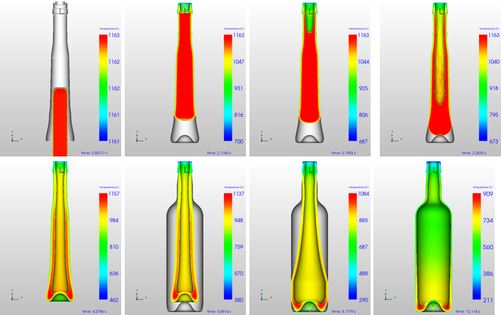
Figure 5: Time steps for C1-0: symmetrically loading
Some single time steps for Case C1-0 are shown in Figure 5. The color is the temperature in °C. The final thickness distribution is shown in Figure 6. As temperature is homogeneous for the initial gob and loading is symmetrically, all results are symmetrically as well.
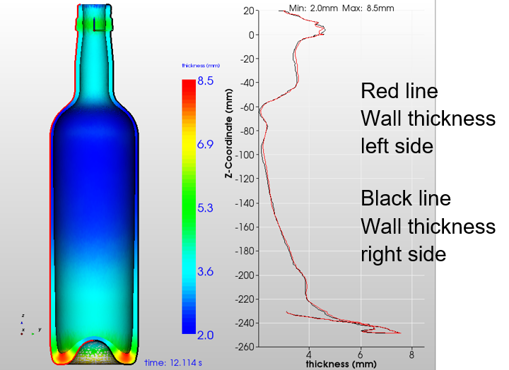
Figure 6: Wall thickness for C1-0: symmetrically loading
If the initial gob position is 2 mm displaced from the center axis, the gob will touch the blank mold wall not symmetrically and a time shift for the contact time occur from left to right side of the gob (see Figure 7). Glass parts which are longer in contact with cold molds are cooling down faster and as a result the wall thickness increases. The final wall thickness distribution is plotted in Figure 8 and there is only a small difference between the left and right wall thickness of 0.25 mm.
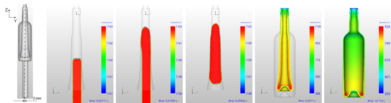
Figure 7: C1-1 Time steps: Loading 2 mm displaced
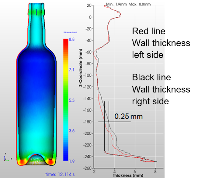
Figure 8: C1-1 Thickness: Loading 2 mm displaced
Next step is to compute the C1-2 case, where temperature difference in the initial gob is ∆T= 72 °C initially. Some images of the temperature at different time steps are shown in Figure 9. As one can see during final blowing the glass is blown to the right side of the blow mold and the flow is completely non-symmetric. Interesting to mention is, that the gob was initially colder on the left side and one would expect that in the final container the left side is thicker as well.
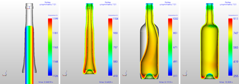
Figure 9: C1-2 Time steps: gob-∆T= 73°C difference
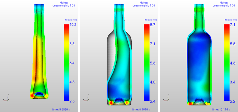
Figure 10: C1-2 Thickness: gob-∆T= 73°C
But referring to Figure 10 one can see that the container is much thicker on the right side. This is understandable if the thickness distribution in the parison is considered. As one can see in Figure 10 (left image) the left side is much thicker than the right side. This is what we expected, but during final blow the flow is always directed in that direction where the lowest resistance occurs. For that reason the complete glass parison moves in the direction with the smallest wall thickness and highest temperature and as a result the wall thickness is higher on the right side.
Due to the inhomogeneous gob temperature the maximum wall thickness at the left side is 2.2 mm whereas on the right side 4.6 mm is computed. Thus, a temperature gradient of 73°C within the gob generates a wall thickness difference of 2.4 mm. If it is allowed to make a linear approximation, one can say, that 1 °C temperature gradient (perpendicular to the gob axis) will produce 0.3 mm thickness differences in the final wall thickness of this container.
The conditions for the container C2 are:
Case C2-0
Symmetrical loading with homogeneous gob temperature,
Case C2-1
Loading with homogeneous gob temperature, but the initial gob position is 5 mm displaced from the center axis.
Case C2-2
Gob loading position is centered, but the initial gob temperature is non-homogeneous. The gob temperature starts with 1134 °C on the left side und increases to 1184 °C on the right side. The maximum temperature difference in the gob is ∆T=50 °C.
Case C2-3
Gob loading position is centered, but the initial gob temperature is non-homogeneous. The gob temperature starts with 1109 °C on the left side und increases to 1209 °C on the right side. The maximum temperature difference in the gob is ∆T=100 °C.
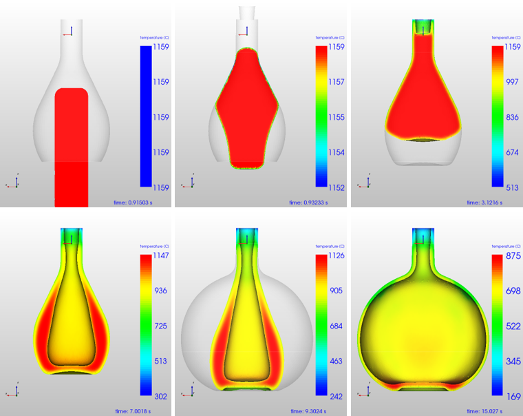
Figure 11: Time steps for C2-0: symmetrical loading
In Figure 11 the single time steps for Case C2-0 are shown and the color is the temperature in °C. The final thickness distribution is shown in Figure 12. As temperature is homogeneous for the initial gob and loading is symmetrical, all results are symmetrical as well.
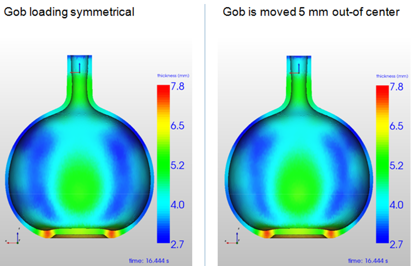
Figure 12: Comparison wall thickness for C2-0 and C2-1
The initial gob position for Case C2-1 is 5 mm displaced from the center axis and the temperature time step images are shown in Figure 14, whereas the corresponding wall thickness is plotted in Figure 13. Same as for the C1-1 case the final wall thickness distribution shows only a small difference between the left and right wall thickness of 0.25 mm.
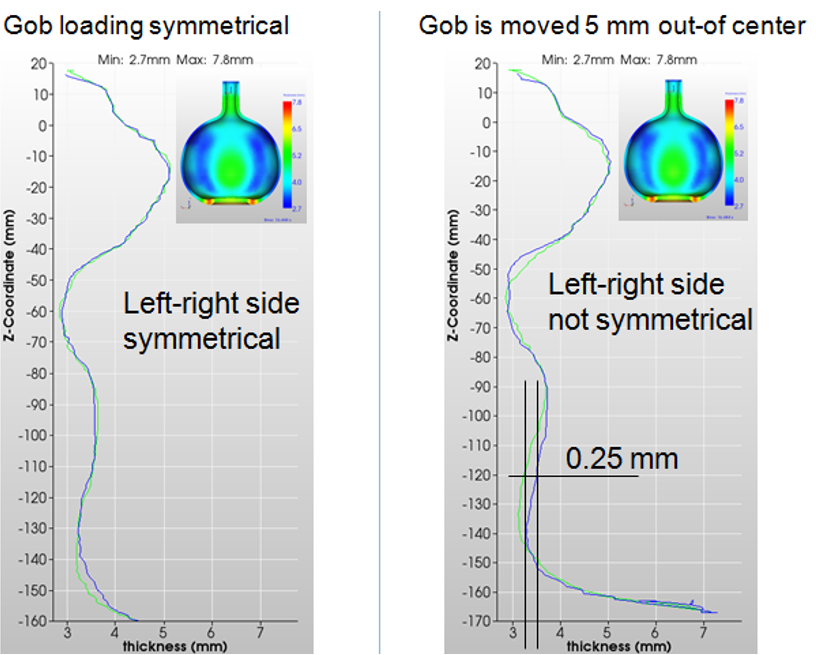
Figure 13: XY-plot wall thickness for C2-0 and C2-1
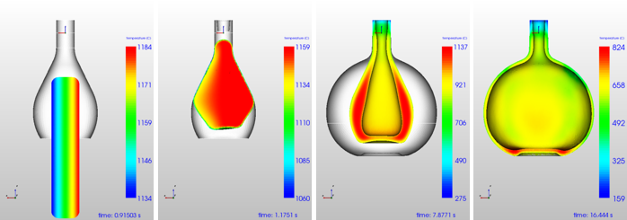
Figure 14: C2-2 Time steps: gob-∆T= 50°C
The results of the case C2-2 and C2-3 computations are shown in Figure 15 and Figure 16. Temperature differences in the gob, here perpendicular to the gob axis do have a higher impact on the final wall thickness distribution than the non-symmetric loading. For this container a temperature difference in the initial gob of ∆T=50 °C generates a wall thickness difference from left to right of 0.9 mm and a gob ∆T of 100 °C produces a wall thickness difference from left to right of 1.4 mm.
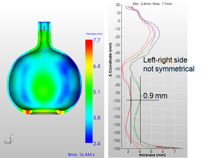
Figure 15: Wall thickness for C2-2: gob-∆T= 50°C
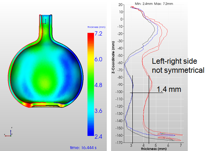
Figure 16: Wall thickness for C2-3: gob-∆T= 100°C
Summary
Nogrid software allows glass container forming processes to be simulated in full 3D and in a very practicable time. In this paper two containers were investigated regarding non-symmetric gob loading and inhomogeneous gob temperature distribution. As most of the results are coupled with the specific container design, it can be concluded that the influence of temperature differences in the gob is much more important for the final container wall thickness distribution than a gob loading displaced from the center axis.
Stärken der Nogrid Software
Unsere Stärke ist das schnelle Preprocessing, da unsere Software auf einer gitterfreien Methode basiert - es muss kein Netz für das Fluidvolumen in 3D oder für die Fluidfläche in 2D generiert werden. Dies führt zu einer besonders kurzen Modellierungszeit (auch für komplizierte Modelle), so dass Sie im Vergleich zu gitterbasierten CFD-Softwareprodukten viel Zeit sparen können. Die gitterfreie Methode ist stark bei der Berechnung von bewegten Teilen oder bei der Berechnung von komplexen freien Oberflächen.
Wie Sie im Bild unten sehen können, benötigt man für die Ränder der Geometrie nach wie vor ein Netz, damit die inneren finiten Punkte den Rand detektieren können. Die Ränder müssen also vernetzt werden und die finiten Punkte im Inneren werden während der Simulation automatisch generiert.
Wie Sie im Bild unten sehen können, benötigt man für die Ränder der Geometrie nach wie vor ein Netz, damit die inneren finiten Punkte den Rand detektieren können. Die Ränder müssen also vernetzt werden und die finiten Punkte im Inneren werden während der Simulation automatisch generiert.
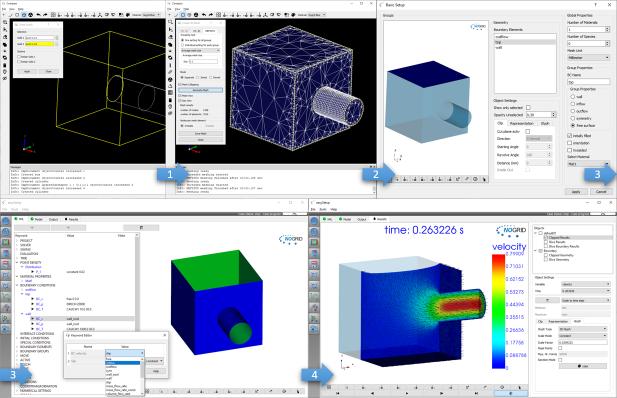
Einfache und schnelle Modellierung: Geometrie erzeugen und Ränder vernetzen, Fall aufsetzen und Simulation starten
Was kann die NOGRID Strömungssimulationssoftware für Sie tun?
Verlässliche industrielle Prozesse sprechen für sich und sind verantwortlich für den Erfolg eines Unternehmens. Für viele Prozesse spielt das Strömungsverhalten des Fluids eine wichtige Rolle für den Erfolg. Da industrielle Designs oft sehr komplex sind, gibt es verschiedene Faktoren, die in Fluidströmungs-Anwendungen wichtig sein können. Durch eine CFD-Simulation mit einer professionellen Software können Sie Ihre Prozessleistung simulieren und relevante Parameter berücksichtigen: Die Anwendung von NOGRIDs numerischer Strömungssimulationssoftware ermöglicht es Ihnen, die Fluidströmung, den Wärme- und Massenübergang sowie eventuell stattfindende chemische Reaktionen vorherzusagen, zu analysieren und zu kontrollieren und gibt Ihnen die Möglichkeit, Ihre Prozessleistung zu optimieren. Dadurch erhalten Sie eine Basis für bessere Design-Entscheidungen.
Die Strömungssimulationssoftware von NOGRID ist ein gitterfreies Tool mit erstaunlicher Flexibilität, Genauigkeit, Zuverlässigkeit und Robustheit. Die Software liefert qualitativ hochwertige Ergebnisse für ein weites Feld von Fluidströmungs-Anwendungen.
Warum sollten Sie sich für NOGRID Strömungssimulationssoftware entscheiden?
Zusätzlich zum Testen und Experimentieren hilft die NOGRID Strömungssimulationssoftware, die Bewertung Ihres Designs zu verbessern und den Erfolg Ihres industriellen Prozesses zu steigern. Zu lernen, wie sich die Fluidströmung verhalten wird und wie sicher industrielle Prozesse oder Prozessschritte funktionieren, lässt Ihr Wissen von Simulation zu Simulation wachsen. Sie bekommen ein besseres Verständnis für Ihre Prozesse, was wiederum zu enormen Einsparungen von Herstellungskosten und - zeit und gleichzeitig zu einem Endprodukt von hoher Qualität führt. Durch Simulation erhalten Sie bessere Konstruktions- und Betriebsparameter, steigende Planungssicherheit und Sie sparen Zeit und Geld dadurch, dass Sie Ihr Produkt schneller auf den Markt bringen können.
Training
In unserem zwei-Tage Trainingskurs werden Sie lernen, wie man die NOGRID CFD/CAE Software effizient einsetzt. Unser technischer Support hat Erfahrungen in vielen Disziplinen und kann Ihnen zeigen, wie man schwierige Fälle bewertet, behandelt und löst.
Für mehr Details bitte hier weiterlesen: Trainingskurse →
Technischer Support
Wir bieten den kompletten technischen Software Support an. Von der ersten Minute an, ab der Sie die Software nutzen, können Sie uns über Telefon oder E-Mail erreichen. Schreiben Sie uns, wir sind Ihnen gerne behilflich.
Für mehr Details bitte hier weiterlesen: Software Support →
Service
Oft sind Zeit und Ressourcen knapp bemessen, so dass die Vergabe von Simulationsaufgaben eine attraktive Möglichkeit sein kann, um schnell und kostengünstig anstehende Aufgaben zu bearbeiten. Basierend auf unserem Know-how können wir eine Fülle von Serviceleistungen auf dem Gebiet der Simulation von Strömungen anbieten.
Wir modellieren und entwickeln für Sie. Sie brauchen hierfür keine NOGRID-Software Lizenz zu kaufen. Wir bieten Ihnen einen individuellen Berechnungsservice für Ihre Verfahren und Prozesse an, der genau auf Ihre Wünsche zugeschnitten ist.
Für mehr Details bitte hier weiterlesen: Simulation Services →